Examples#
The examples/ directory contains a collection of scripts demonstrating various applications of spicex.
current_source_with_resistor#
See on GitHub: examples/current_source_with_resistor
README:
# Current Source with Resistor

Philip Mocz (2026)

Simple current source with resistor


## Circuit

```
 n1+------------+
   |            |
 [ I=1mA ]    [ R=1kΩ ]
   |            |
 n0+------------+
```


## Usage

```console
python current_source_with_resistor.py
```
Script:
import jax
import spicex

# switch on for double precision
jax.config.update("jax_enable_x64", True)

"""
Current source driving a resistor.

Philip Mocz (2026)

Usage:
  python current_source_with_resistor.py
"""


def main():
    circuit = spicex.Circuit(n_nodes=2)
    circuit.add_current_source(0, 1, 1e-3)  # 1 mA from ground to node 1
    circuit.add_resistor(1, 0, 1e3)  # 1 kΩ from node 1 to ground

    v_nodes, i_vsrc, *_ = circuit.solve()

    print(f"Node voltages: {v_nodes}")
    print(f"Voltage source currents: {i_vsrc}")

    return v_nodes, i_vsrc


if __name__ == "__main__":
    main()
maximum_power_transfer#
See on GitHub: examples/maximum_power_transfer
README:
# Maximum Power Transfer

Philip Mocz (2026)

Autodiff through the circuit solver to find the load resistance R_L
that maximizes power delivered to it from a voltage source


## Circuit

```
 n1+----[ R_s=1kΩ ]----+n2
   |                   |
 [ V=10V ]        [ R_L (optimized) ]
   |                   |
 n0+-------------------+
```


## Usage

```console
python maximum_power_transfer.py
```


## Result

Analytic result: max power transfer when `R_L = R_s`

Maximum power: `P_max = V_s^2 / (4 * R_s) = 25 mW`


## Reference

https://en.wikipedia.org/wiki/Maximum_power_transfer_theorem
Script:
import jax
import jax.numpy as jnp
import spicex

# switch on for double precision
jax.config.update("jax_enable_x64", True)

"""
Maximum Power Transfer

Philip Mocz (2026)

Usage:
  python maximum_power_transfer.py
"""

V_S = 10.0  # source voltage (V)
R_S = 1e3  # source resistance (Ohm)


def power_in_load(log_R_L):
    """Power delivered to the load resistor R_L."""
    R_L = jnp.exp(log_R_L)
    circuit = spicex.Circuit(n_nodes=3)
    circuit.add_voltage_source(0, 1, V_S)
    circuit.add_resistor(1, 2, R_S)
    circuit.add_resistor(2, 0, R_L)
    v_nodes, *_ = circuit.solve()
    return v_nodes[2] ** 2 / R_L


def main():
    @jax.jit
    def loss_fn(log_R_L):
        return -power_in_load(log_R_L)

    log_R_L = jnp.log(100.0)

    log_R_L_opt, _ = spicex.optimize(log_R_L, loss_fn, max_iter=100, tol=1e-8)

    R_L_opt = jnp.exp(log_R_L_opt)
    P_opt = power_in_load(log_R_L_opt)
    P_analytic = V_S**2 / (4.0 * R_S)

    print(f"Optimal R_L:   {float(R_L_opt):.2f} Ohm  (analytic: {R_S:.0f} Ohm)")
    print(
        f"Max power: {float(P_opt) * 1e3:.4f} mW  (analytic: {P_analytic * 1e3:.0f} mW)"
    )

    return R_L_opt, P_opt


if __name__ == "__main__":
    main()
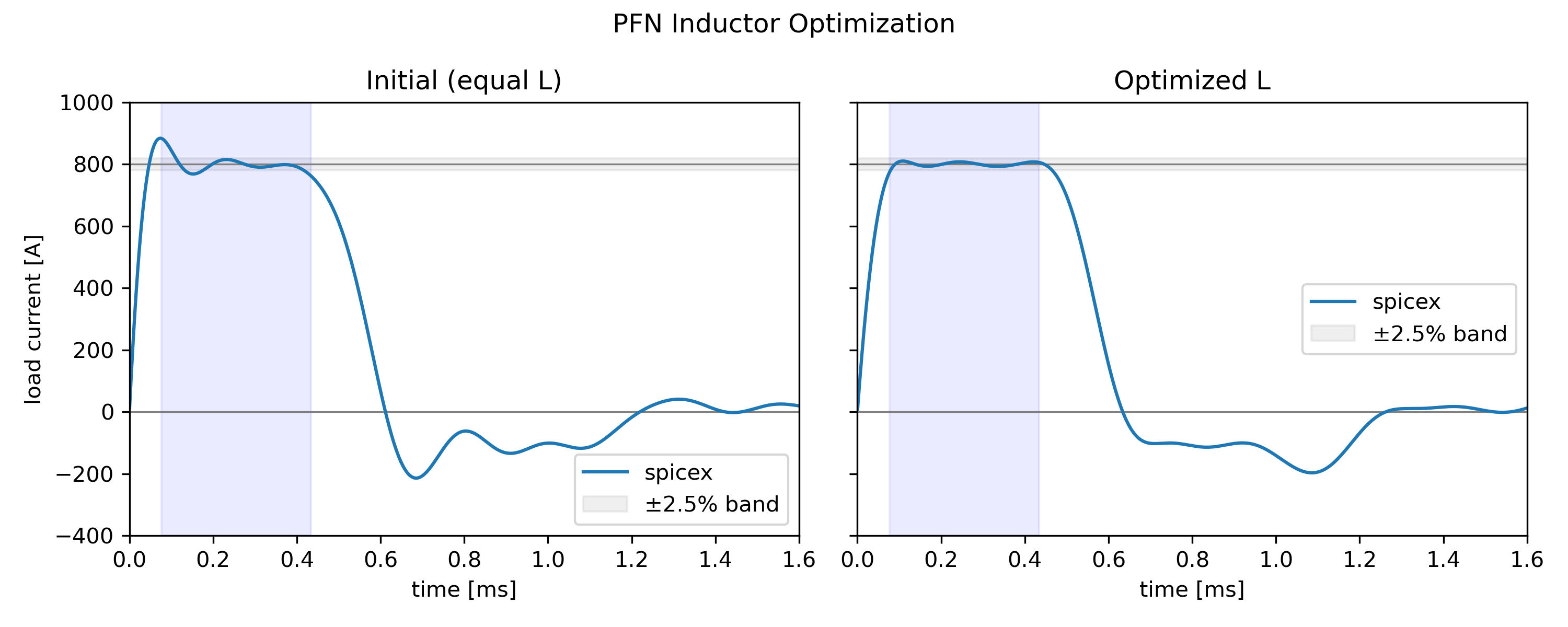
pfn_optimize#
See on GitHub: examples/pfn_optimize
README:
# PFN Inductor Optimization
Philip Mocz (2026)
Optimize the inductor distribution of a 5-section PFN to maximize pulse flatness,
using automatic differentiation through the transient circuit simulation.
## Circuit
```
n1+--[ L1 ]--+n2--[ L2 ]--+n3--[ L3 ]--+n4--[ L4 ]--+n5--[ L5 ]--+n6
| | | | | |
| [ C1 ] [ C2 ] [ C3 ] [ C4 ] [ C5 ]
| | | | | |
[ R_load ] +n7 +n8 +n9 +n10 +n11
| | | | | |
| [ R_esr ] [ R_esr ] [ R_esr ] [ R_esr ] [ R_esr ]
| | | | | |
n0+----------+------------+------------+------------+------------+
```
Same topology as `examples/pfn_type_b`, but all five capacitors are equal
(C = 390 µF each) and the five inductor values are the free parameters.
The load (100 mΩ) connects at the left output terminal.
All capacitors are pre-charged to V0; all inductor currents are zero at t = 0.
## Usage
```console
python pfn_optimize.py [--plot]
```
## Optimization
The inductor values are parameterized via a log-softmax so that all L_k > 0
and sum(L_k) = L_total (pulse duration is preserved):
```
L_k = L_total * softmax(w)_k
```
The loss function is the normalized RMS deviation of the load current from
I_target over the flat-top window (15%–85% of the pulse duration):
```
loss = sum_t[ mask(t) * (I(t) - I_target)^2 ] / (N_flat * I_target^2)
```
Gradients are computed with JAX automatic differentiation through the full
transient simulation, and weights are updated with `spicex.optimize()`.
## Result

Script:
import argparse
import jax
import jax.numpy as jnp
import spicex

# switch on for double precision
jax.config.update("jax_enable_x64", True)

"""
PFN Inductor Optimization

Philip Mocz (2026)

Optimize the 5 inductor values of a PFN to maximize pulse flatness,
using automatic differentiation through the transient circuit simulation.

The inductor distribution is parameterized via a log-softmax so all
L_k > 0 and sum(L_k) = L_total (pulse duration is preserved).

c.f. `examples/pfn_type_b/pfn_type_b.py`

Usage:
  python pfn_optimize.py [--plot]
"""

# Fixed circuit parameters
L_total = 33.4e-6  # total inductance (H), shared equally at init
C_section = 390e-6  # equal section capacitance (F)  ~1950 µF total
C_total = 5 * C_section
R_esr = 5e-3  # 5 mΩ ESR per capacitor branch
R_load = 100e-3  # 100 mΩ matched load

Z0 = float(jnp.sqrt(L_total / C_total))  # ~0.131 Ω
I_target = 800.0
V0 = I_target * (Z0 + R_load)  # initial charge voltage
T_pulse = 2.0 * float(jnp.sqrt(L_total * C_total))  # ~0.51 ms

# Flat-top window
T_FLAT_LO = 0.15 * T_pulse
T_FLAT_HI = 0.85 * T_pulse

# Simulation parameters
t_end = 1.6e-3  # 1.6 ms
dt = 500e-9  # 500 ns


def simulate(log_L_weights):
    """Run transient simulation for given inductor log-weights.

    log_L_weights : shape (5,)
        Unnormalized log weights; Ls = L_total * softmax(log_L_weights)

    Returns
    -------
    t        : shape (n_steps,)
    i_load   : shape (n_steps,)  load current in A
    """
    Ls = L_total * jax.nn.softmax(log_L_weights)

    circuit = spicex.Circuit(n_nodes=12)

    # Series inductors along top rail
    circuit.add_inductor(1, 2, Ls[0])
    circuit.add_inductor(2, 3, Ls[1])
    circuit.add_inductor(3, 4, Ls[2])
    circuit.add_inductor(4, 5, Ls[3])
    circuit.add_inductor(5, 6, Ls[4])

    # Shunt branches: Ck + R_esr  (equal caps)
    circuit.add_capacitor(2, 7, C_section)
    circuit.add_resistor(7, 0, R_esr)
    circuit.add_capacitor(3, 8, C_section)
    circuit.add_resistor(8, 0, R_esr)
    circuit.add_capacitor(4, 9, C_section)
    circuit.add_resistor(9, 0, R_esr)
    circuit.add_capacitor(5, 10, C_section)
    circuit.add_resistor(10, 0, R_esr)
    circuit.add_capacitor(6, 11, C_section)
    circuit.add_resistor(11, 0, R_esr)

    # Load at output terminal
    circuit.add_resistor(1, 0, R_load)

    # Initial conditions: capacitor nodes at V0, all else at 0
    v0 = jnp.array([0.0, 0.0, V0, V0, V0, V0, V0, 0.0, 0.0, 0.0, 0.0, 0.0])
    i_L0 = jnp.zeros(5)

    t, v_nodes, *_ = circuit.solve_transient(t_end=t_end, dt=dt, v0=v0, i_L0=i_L0)
    return t, v_nodes[:, 1] / R_load


@jax.jit
def loss_fn(log_L_weights):
    """Normalized RMS deviation from I_target over the flat-top window."""
    t, i_load = simulate(log_L_weights)
    mask = (t >= T_FLAT_LO) & (t <= T_FLAT_HI)
    n_flat = jnp.sum(mask)
    return jnp.sum(mask * (i_load - I_target) ** 2) / (n_flat * I_target**2)


def flatness_pct(t, i_load):
    """Peak-to-peak flatness as ± % of mean in flat-top window."""
    mask = (t >= T_FLAT_LO) & (t <= T_FLAT_HI)
    i_flat = i_load[mask]
    i_mean = float(jnp.mean(i_flat))
    return float(100.0 * jnp.max(jnp.abs(i_flat - i_mean)) / i_mean)


def main():
    log_L_weights_init = jnp.zeros(5)  # equal inductors

    print("Optimizing inductor distribution for maximum flatness...")
    print()
    log_L_weights_opt, _ = spicex.optimize(
        log_L_weights_init, loss_fn, max_iter=200, tol=1e-10
    )

    t, i_before = simulate(log_L_weights_init)
    t, i_after = simulate(log_L_weights_opt)

    L_init = L_total * jax.nn.softmax(log_L_weights_init)
    L_opt = L_total * jax.nn.softmax(log_L_weights_opt)

    print()
    print(f"  {'':20s}  {'Initial':>12s}  {'Optimized':>12s}")
    print("  " + "-" * 50)
    for k in range(5):
        print(
            f"  L{k + 1}                      "
            f"  {float(L_init[k]) * 1e6:10.2f} µH"
            f"  {float(L_opt[k]) * 1e6:10.2f} µH"
        )
    print("  " + "-" * 50)
    print(
        f"  Peak current              "
        f"  {float(jnp.max(i_before)):10.1f} A "
        f"  {float(jnp.max(i_after)):10.1f} A"
    )
    print(
        f"  Flatness (±%)             "
        f"  {flatness_pct(t, i_before):10.2f} % "
        f"  {flatness_pct(t, i_after):10.2f} %"
    )

    return t, i_before, i_after


def plot(t, i_before, i_after):
    import matplotlib.pyplot as plt

    fig, axes = plt.subplots(1, 2, figsize=(10, 4), sharey=True)

    for ax, i_load, title in zip(
        axes, [i_before, i_after], ["Initial (equal L)", "Optimized L"]
    ):
        ax.axhspan(
            I_target * 0.975,
            I_target * 1.025,
            alpha=0.12,
            color="gray",
            label="±2.5% band",
        )
        ax.axhline(I_target, color="gray", linewidth=0.8, linestyle="-")
        ax.axhline(0, color="gray", linewidth=0.8, linestyle="-")
        ax.axvspan(T_FLAT_LO * 1e3, T_FLAT_HI * 1e3, alpha=0.08, color="blue")
        ax.plot(t * 1e3, i_load, linewidth=1.5, label="spicex")
        ax.set_xlim(0, t_end * 1e3)
        ax.set_ylim(-400, 1000)
        ax.set_xlabel("time [ms]")
        ax.set_title(title)
        ax.legend()

    axes[0].set_ylabel("load current [A]")
    fig.suptitle("PFN Inductor Optimization")
    plt.tight_layout()
    plt.savefig("pfn_optimize.png", dpi=300)
    plt.show()


if __name__ == "__main__":
    parser = argparse.ArgumentParser()
    parser.add_argument("--plot", action="store_true", help="Plot load current vs time")
    args = parser.parse_args()

    t, i_before, i_after = main()

    if args.plot:
        plot(t, i_before, i_after)
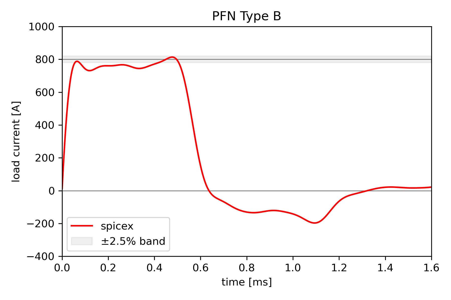
pfn_type_b#
See on GitHub: examples/pfn_type_b
README:
# PFN Type B
Philip Mocz (2026)
Transient simulation of a Type B Pulse-Forming Network (PFN) discharge
## Circuit
```
n1+--[ L1 ]--+n2--[ L2 ]--+n3--[ L3 ]--+n4--[ L4 ]--+n5--[ L5 ]--+n6
| | | | | |
| [ C1 ] [ C2 ] [ C3 ] [ C4 ] [ C5 ]
| | | | | |
[ R_load ] +n7 +n8 +n9 +n10 +n11
| | | | | |
| [ R_esr ] [ R_esr ] [ R_esr ] [ R_esr ] [ R_esr ]
| | | | | |
n0+----------+------------+------------+------------+------------+
```
Five series inductors along the top rail; five shunt capacitor + ESR branches.
The load (100 mΩ) connects at the left output terminal.
All capacitors are pre-charged to V0; all inductor currents are zero at t = 0.
## Usage
```console
python pfn_type_b.py [--plot]
```
## Transient Analysis
When the switch closes at t = 0, the PFN discharges into R_load.
The Thevenin equivalent of the network presents V_th = V0/2 and Z_th = Z0,
so the flat-top load current is approximately:
```
I_flat = V0 / (Z0 + R_load)
```
The non-uniform L and C values shape the current pulse to be flat
within ±2.5% over the central portion of the pulse duration.
## Result

## Reference
https://blog.wolfram.com/2022/05/06/building-a-pulse-forming-network-with-the-wolfram-language/
Script:
import argparse
import jax
import jax.numpy as jnp
import spicex

# switch on for double precision
jax.config.update("jax_enable_x64", True)

"""
PFN Type B

Philip Mocz (2026)

Usage:
  python pfn_type_b.py [--plot]
"""

# Component values
L1, L2, L3, L4, L5 = 6.6e-6, 5.4e-6, 5.6e-6, 6.5e-6, 9.3e-6  # inductances (H)
C1, C2, C3, C4, C5 = 250e-6, 250e-6, 300e-6, 350e-6, 800e-6  # capacitances (F)
R_esr = 5e-3  # 5 mΩ equivalent series resistance (ESR) for each capacitor branch
R_load = 100e-3  # 100 mΩ matched load

# Characteristic impedance and initial charge voltage
L_total = L1 + L2 + L3 + L4 + L5  # 33.4 µH
C_total = C1 + C2 + C3 + C4 + C5  # 1950 µF
Z0 = float(jnp.sqrt(L_total / C_total))  # ~ 0.131 Ω

# Calibrate V0 so the flat-top current ~ 800 A into R_load
I_target = 800.0
V0 = I_target * (Z0 + R_load)

# Pulse duration: T ~ 2*sqrt(L_total * C_total) ~ 0.51 ms
T_pulse = 2.0 * float(jnp.sqrt(L_total * C_total))

# Simulation parameters
t_end = 1.6e-3  # 1.6 ms
dt = 500e-9  # 500 ns


def main():
    circuit = spicex.Circuit(n_nodes=12)

    # Series inductors along top rail
    circuit.add_inductor(1, 2, L1)
    circuit.add_inductor(2, 3, L2)
    circuit.add_inductor(3, 4, L3)
    circuit.add_inductor(4, 5, L4)
    circuit.add_inductor(5, 6, L5)

    # Shunt branches: Ck + R_esr
    circuit.add_capacitor(2, 7, C1)
    circuit.add_resistor(7, 0, R_esr)
    circuit.add_capacitor(3, 8, C2)
    circuit.add_resistor(8, 0, R_esr)
    circuit.add_capacitor(4, 9, C3)
    circuit.add_resistor(9, 0, R_esr)
    circuit.add_capacitor(5, 10, C4)
    circuit.add_resistor(10, 0, R_esr)
    circuit.add_capacitor(6, 11, C5)
    circuit.add_resistor(11, 0, R_esr)

    # Load at output terminal
    circuit.add_resistor(1, 0, R_load)

    # Initial conditions:
    #   PFN nodes n2-n6 at V0 (capacitors fully charged).
    #   n1 at 0 V (output terminal was isolated before switch closed at t=0).
    #   Intermediate nodes n7-n11 at 0 V (no pre-discharge current through ESR).
    #   All inductor currents zero (no current before switch).
    v0 = jnp.array([0.0, 0.0, V0, V0, V0, V0, V0, 0.0, 0.0, 0.0, 0.0, 0.0])
    i_L0 = jnp.zeros(5)

    t, v_nodes, i_vsrc, i_inductor, i_capacitor = circuit.solve_transient(
        t_end=t_end, dt=dt, v0=v0, i_L0=i_L0
    )

    i_load = v_nodes[:, 1] / R_load  # load current (A)

    # Metrics
    i_peak = float(jnp.max(i_load))

    # Flat-top: central region 15%--85% of T_pulse
    t_flat_lo, t_flat_hi = 0.15 * T_pulse, 0.85 * T_pulse
    mask = (t >= t_flat_lo) & (t <= t_flat_hi)
    i_flat = i_load[mask]
    i_mean = float(jnp.mean(i_flat))
    flat_pct = float(100.0 * jnp.max(jnp.abs(i_flat - i_mean)) / i_mean)

    # Rise time: 10% --> 90% of peak
    idx10 = int(jnp.argmax(i_load >= 0.10 * i_peak))
    idx90 = int(jnp.argmax(i_load >= 0.90 * i_peak))
    rise_us = float((t[idx90] - t[idx10]) * 1e6)

    print(f"Z0          = {Z0 * 1e3:.2f} mΩ  (PFN characteristic impedance)")
    print(f"V0          = {V0:.1f} V  (initial charge voltage)")
    print(f"T_pulse     = {T_pulse * 1e3:.3f} ms  (approx. pulse duration)")
    print()
    print(f"Peak current : {i_peak:.1f} A")
    print(f"Rise time    : {rise_us:.1f} µs  (10%-->90% of peak)")
    print(
        f"Flat-top mean: {i_mean:.1f} A  (t = {t_flat_lo * 1e3:.2f}--{t_flat_hi * 1e3:.2f} ms)"
    )
    print(f"Flatness     : ±{flat_pct:.2f}%")

    return t, v_nodes, i_load


def plot(t, v_nodes, i_load):
    import matplotlib.pyplot as plt

    fig, ax = plt.subplots(figsize=(6, 4))

    # ±2.5% flatness band around target
    ax.axhspan(
        I_target * 0.975, I_target * 1.025, alpha=0.12, color="gray", label="±2.5% band"
    )
    ax.axhline(I_target, color="gray", linewidth=0.8, linestyle="-")
    ax.axhline(0, color="gray", linewidth=0.8, linestyle="-")

    ax.plot(t * 1e3, i_load, color="r", linewidth=1.5, label="spicex")

    ax.set_xlim(0, t_end * 1e3)
    ax.set_ylim(-400, 1000)
    ax.set_xlabel("time [ms]")
    ax.set_ylabel("load current [A]")
    ax.set_title("PFN Type B")
    ax.legend()
    plt.tight_layout()
    plt.savefig("pfn_type_b.png", dpi=300)
    plt.show()


if __name__ == "__main__":
    parser = argparse.ArgumentParser()
    parser.add_argument("--plot", action="store_true", help="Plot load current vs time")
    args = parser.parse_args()

    t, v_nodes, i_load = main()

    if args.plot:
        plot(t, v_nodes, i_load)
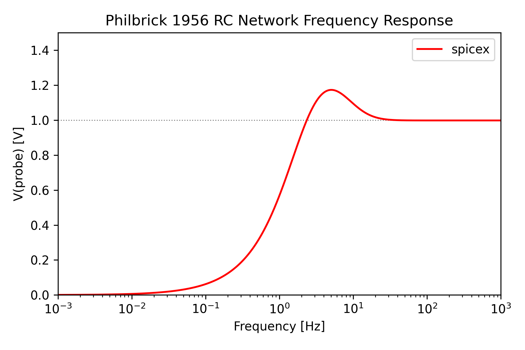
philbrick_1956#
See on GitHub: examples/philbrick_1956
README:
# Philbrick 1956 RC Network
Philip Mocz (2026)
AC frequency response of the three-resistor, three-capacitor RC network
patented by Philbrick in 1956.
## Circuit
```
n3 (probe, V)
|
n2+(bus)--+---[ C1 10nF ]-----+---------[ RLOAD 100Meg ]---+
| | | |
| | [ R2 3.3Meg ] |
| | | |
| | | |
| +---[ C2 20nF ]-----+n4 |
| | | |
| | [ R3 1.0Meg ] |
| | | |
| | | |
| +---[ C3 50nF ]-----+n5 |
| | |
[ RSRC 1k ] [ R4 510k ] |
| | |
n1 n0+----------------------------+
|
[ VSRC 1V ]
|
n0
```
The R2-R3-R4 chain is a single vertical spine on the right; n4 and n5 are
each a single junction where C2 and C3 tap into that spine (not separate
nodes) — R2 runs from n3 down to n4, R3 from n4 down to n5, R4 from n5
down to ground. n2 is the bus feeding all three capacitors' left plates
from RSRC.
Node 2 (the RSRC/C1/C2/C3 bus) reaches the R2-R3-R4 ladder and probe node
n3 only through capacitors, so the network has no DC path: gain -> 0 as
f -> 0. At high frequency the capacitors short the ladder onto the bus
and, since RLOAD >> RSRC, gain -> 1. In between, the three-section CR
ladder produces a resonance-like peak above unity.
## Usage
```console
python philbrick_1956.py [--plot]
```
## Parameters
| Symbol | Value |
|--------|-------|
| RSRC | 1 kΩ |
| C1 | 10 nF |
| C2 | 20 nF |
| C3 | 50 nF |
| R2 | 3.3 MΩ |
| R3 | 1.0 MΩ |
| R4 | 510 kΩ |
| RLOAD | 100 MΩ |
## AC Analysis
`Circuit.solve_ac(omega)` performs a phasor (sinusoidal steady-state)
solve at each angular frequency, folding capacitors and inductors
directly into the admittance matrix (`Y_C = jωC`). The frequency sweep
uses `spicex.sweep`, which `jax.vmap`s the per-frequency solve over a
log-spaced array of 601 points from 1 mHz to 1 kHz (six decades).
## Result
For a 1 V input, the simulated gain peaks at **1.17 V near 5.0 Hz**, and
exceeds unity for roughly **2.4 Hz to 37 Hz**, closely matching the shape
described for this circuit (peak ≈ 1.19 V at ≈ 4.64 Hz, gain > 1 for
≈ 2-20 Hz) — the small numeric difference is expected since the
component values are rounded to two significant figures.

Script:
import argparse
import jax
import jax.numpy as jnp
import spicex

jax.config.update("jax_enable_x64", True)

"""
Philbrick 1956 RC Network

AC frequency response of the three-resistor, three-capacitor RC network
patented by Philbrick in 1956. A 1 V source drives RSRC into a bus shared
by three parallel R-C branches feeding a resistive ladder (R2-R3-R4) that
is probed at V and terminated by RLOAD.

The bus reaches the ladder only through capacitors, so the network has no
DC path: gain -> 0 as f -> 0. At high frequency the capacitors short the
ladder onto the bus and, since RLOAD >> RSRC, gain -> 1. In between, the
three-section CR ladder produces a resonance-like peak above 1.

Philip Mocz (2026)

Usage:
  python philbrick_1956.py [--plot]
"""

RSRC = 1e3  # source resistance (Ohm)
C1 = 10e-9  # F
C2 = 20e-9  # F
C3 = 50e-9  # F
R2 = 3.3e6  # Ohm
R3 = 1.0e6  # Ohm
R4 = 510e3  # Ohm
RLOAD = 100e6  # Ohm
V_S = 1.0  # source amplitude (V)

F_MIN = 1e-3  # Hz
F_MAX = 1e3  # Hz
N_FREQ = 601


def build_circuit():
    # Nodes: 0=GND, 1=VSRC+, 2=RSRC/C1/C2/C3 bus,
    #        3=probe V (C1-R2-RLOAD), 4=R2-C2-R3 junction, 5=R3-C3-R4 junction
    circuit = spicex.Circuit(n_nodes=6)
    circuit.add_voltage_source(0, 1, V_S)
    circuit.add_resistor(1, 2, RSRC)
    circuit.add_capacitor(2, 3, C1)
    circuit.add_capacitor(2, 4, C2)
    circuit.add_capacitor(2, 5, C3)
    circuit.add_resistor(3, 4, R2)
    circuit.add_resistor(4, 5, R3)
    circuit.add_resistor(5, 0, R4)
    circuit.add_resistor(3, 0, RLOAD)
    return circuit


def main():
    freq = jnp.logspace(jnp.log10(F_MIN), jnp.log10(F_MAX), N_FREQ)
    omega = 2.0 * jnp.pi * freq

    def probe_at(w):
        v_nodes, _ = build_circuit().solve_ac(w)
        return v_nodes[3]

    v_probe = spicex.sweep(probe_at, omega)
    gain = jnp.abs(v_probe)

    peak_idx = int(jnp.argmax(gain))
    print(
        f"Peak gain: {float(gain[peak_idx]):.3f} V at f = {float(freq[peak_idx]):.3f} Hz"
    )

    above_unity = freq[gain > 1.0]
    if above_unity.size:
        print(
            f"Gain > 1.0 for f in [{float(above_unity[0]):.2f}, "
            f"{float(above_unity[-1]):.2f}] Hz"
        )

    return freq, v_probe


def plot(freq, v_probe):
    import matplotlib.pyplot as plt

    gain = jnp.abs(v_probe)

    fig, ax = plt.subplots(figsize=(6, 4))
    ax.axhline(1.0, color="gray", linewidth=0.8, linestyle=":")
    ax.plot(freq, gain, color="red", label="spicex")
    ax.set_xscale("log")
    ax.set_xlim(float(freq[0]), float(freq[-1]))
    ax.set_ylim(0.0, 1.5)
    ax.set_xlabel("Frequency [Hz]")
    ax.set_ylabel("V(probe) [V]")
    ax.set_title("Philbrick 1956 RC Network Frequency Response")
    ax.legend()
    plt.tight_layout()
    plt.savefig("philbrick_1956.png", dpi=300)
    plt.show()


if __name__ == "__main__":
    parser = argparse.ArgumentParser()
    parser.add_argument(
        "--plot", action="store_true", help="Plot |V(probe)| vs frequency"
    )
    args = parser.parse_args()

    freq, v_probe = main()

    if args.plot:
        plot(freq, v_probe)
resistors_in_parallel#
See on GitHub: examples/resistors_in_parallel
README:
# Resistors in Parallel

Philip Mocz (2026)

Simple resistors in parallel example


## Circuit

```
 n1+----------+----------+
   |          |          |
 [ V=5V ] [ R1=1kΩ ] [ R2=2kΩ ]
   |          |          |
 n0+----------+----------+
```


## Usage

```console
python resistors_in_parallel.py
```
Script:
import jax
import spicex

# switch on for double precision
jax.config.update("jax_enable_x64", True)

"""
Two resistors in parallel with a voltage source

Philip Mocz (2026)

Usage:
  python resistors_in_parallel.py
"""


def main():
    circuit = spicex.Circuit(n_nodes=2)
    circuit.add_voltage_source(0, 1, 5.0)  # 5 V source: ground --> node 1
    circuit.add_resistor(1, 0, 1e3)  # 1 kΩ: node 1 --> ground
    circuit.add_resistor(1, 0, 2e3)  # 2 kΩ: node 1 --> ground
    v_nodes, i_vsrc, *_ = circuit.solve()

    print("Node voltages:", v_nodes)
    print("Current through voltage source:", i_vsrc)

    return v_nodes, i_vsrc


if __name__ == "__main__":
    main()
resistors_in_series#
See on GitHub: examples/resistors_in_series
README:
# Resistors in Series

Philip Mocz (2026)

Simple resistors in series example


## Circuit

```
 n1+----[ R1=1kΩ ]----+n2
   |                   |
 [ V=5V ]          [ R2=2kΩ ]
   |                   |
 n0+-------------------+
```


## Usage

```console
python resistors_in_series.py
```
Script:
import jax
import spicex

# switch on for double precision
jax.config.update("jax_enable_x64", True)

"""
Two resistors in parallel with a voltage source

Philip Mocz (2026)

Usage:
  python resistors_in_series.py
"""


def main():
    circuit = spicex.Circuit(n_nodes=3)
    circuit.add_voltage_source(0, 1, 5.0)  # 5 V source: ground --> node 1
    circuit.add_resistor(1, 2, 1e3)  # 1 kΩ: node 1 --> node 2
    circuit.add_resistor(2, 0, 2e3)  # 2 kΩ: node 2 --> ground
    v_nodes, i_vsrc, *_ = circuit.solve()

    print("Node voltages:", v_nodes)
    print("Current through voltage source:", i_vsrc)

    return v_nodes, i_vsrc


if __name__ == "__main__":
    main()
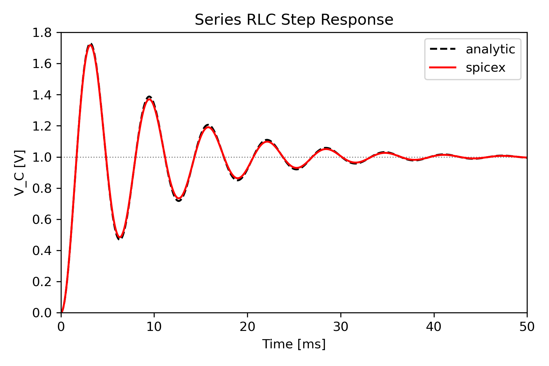
rlc_series#
See on GitHub: examples/rlc_series
README:
# RLC Series Circuit
Philip Mocz (2026)
Transient simulation of a series RLC circuit driven by a 1 V step voltage source
## Circuit
```
n1+---[ L=10mH ]---+n2---[ R=2Ω ]---+n3
| |
[ V=1V ] [ C=100µF ]
| |
n0+---------------------------------+
```
## Usage
```console
python rlc_series.py [--plot]
```
## Parameters
| Symbol | Value | Description |
|--------|-------|-------------|
| ω₀ | 1000 rad/s | Natural frequency 1/√(LC) |
| ζ | 0.1 | Damping ratio R/(2√(L/C)) |
| τ | 10 ms | Envelope time constant 1/(ζω₀) |
| T₀ | 6.28 ms | Oscillation period 2π/ω₀ |
## Transient Analysis
With ζ = 0.1 < 1 the circuit is **underdamped**: the capacitor voltage oscillates
before settling to V_S = 1 V.
Analytic solution:
```
V_C(t) = V_S [1 − e^(−αt)(cos ω_d t + (α/ω_d) sin ω_d t)]
```
where α = ζω₀ = 100 rad/s and ω_d = ω₀√(1−ζ²) ≈ 995 rad/s.
The first overshoot peak occurs at t ≈ π/ω_d ≈ 3.16 ms:
```
V_C_peak = V_S (1 + e^(−απ/ω_d)) ≈ 1.73 V
```
## Result

Script:
import argparse
import jax
import jax.numpy as jnp
import spicex

# switch on for double precision
jax.config.update("jax_enable_x64", True)

"""
RLC Series Circuit

A 1 V voltage source drives a series R-L-C circuit.

  R = 2 Ω,  L = 10 mH,  C = 100 µF
  ω₀ = 1/√(LC) = 1000 rad/s  (f₀ ≈ 159 Hz,  T₀ ≈ 6.28 ms)
  ζ  = R / (2√(L/C)) = 0.1   (underdamped — oscillatory step response)

Analytic capacitor voltage:
  V_C(t) = V_S [1 − e^(−αt)(cos ω_d t + (α/ω_d) sin ω_d t)]
where α = ζω₀,  ω_d = ω₀√(1−ζ²).

Philip Mocz (2026)

Usage:
  python rlc_series.py [--plot]
"""

R = 2.0  # resistance (Ω)
L = 10e-3  # inductance (H)
C = 100e-6  # capacitance (F)
V_S = 1.0  # source voltage (V)
t_end = 50e-3  # 50 ms ~= 5τ  (τ = 1/(ζω₀) = 10 ms)
dt = 0.01e-3  # 0.01 ms ==? 5000 steps, ~628 steps per oscillation period


def main():
    # Nodes: 0=GND, 1=V_source+, 2=L-R junction, 3=R-C junction (cap voltage)
    circuit = spicex.Circuit(n_nodes=4)
    circuit.add_voltage_source(0, 1, V_S)  # 1 V step: GND --> node 1
    circuit.add_inductor(1, 2, L)  # 10 mH: node 1 --> node 2
    circuit.add_resistor(2, 3, R)  # 2 Ω:   node 2 --> node 3
    circuit.add_capacitor(3, 0, C)  # 100 µF: node 3 --> GND

    t, v_nodes, i_vsrc, i_inductor, i_capacitor = circuit.solve_transient(
        t_end=t_end, dt=dt
    )

    # Analytic solution (underdamped series RLC)
    alpha = R / (2.0 * L)  # = ζω₀ = 100 rad/s
    omega0 = 1.0 / jnp.sqrt(L * C)  # = 1000 rad/s
    omega_d = jnp.sqrt(omega0**2 - alpha**2)  # ≈ 994.99 rad/s
    v_analytic = V_S * (
        1.0
        - jnp.exp(-alpha * t)
        * (jnp.cos(omega_d * t) + (alpha / omega_d) * jnp.sin(omega_d * t))
    )

    peak_idx = int(jnp.argmax(v_nodes[:, 3]))
    print(
        f"ω₀ = {float(omega0):.1f} rad/s,  ζ = {R / (2 * float(jnp.sqrt(L / C))):.2f}"
    )
    print(
        f"Peak V_C: {float(v_nodes[peak_idx, 3]):.4f} V at t = {float(t[peak_idx]) * 1e3:.3f} ms"
        f"  (analytic peak ≈ {float(jnp.max(v_analytic)):.4f} V)"
    )
    print()
    print(
        f"{'t (ms)':>8}  {'V_C sim (V)':>12}  {'V_C analytic (V)':>16}  {'err (%)':>8}"
    )
    for k in range(0, len(t), 500):
        sim = float(v_nodes[k, 3])
        ana = float(v_analytic[k])
        err = 100.0 * abs(sim - ana) / (abs(ana) + 1e-12)
        print(f"  {float(t[k]) * 1e3:6.2f}  {sim:12.6f}  {ana:16.6f}  {err:8.4f}")

    return t, v_nodes, i_vsrc, i_inductor, i_capacitor


def plot(t, v_nodes):
    import matplotlib.pyplot as plt

    alpha = R / (2.0 * L)
    omega0 = 1.0 / jnp.sqrt(L * C)
    omega_d = jnp.sqrt(omega0**2 - alpha**2)
    v_analytic = V_S * (
        1.0
        - jnp.exp(-alpha * t)
        * (jnp.cos(omega_d * t) + (alpha / omega_d) * jnp.sin(omega_d * t))
    )

    fig, ax = plt.subplots(figsize=(6, 4))
    ax.axhline(V_S, color="gray", linewidth=0.8, linestyle=":")
    ax.plot(t * 1e3, v_analytic, "--", color="black", label="analytic")
    ax.plot(t * 1e3, v_nodes[:, 3], color="red", label="spicex")
    ax.set_xlim(0, t_end * 1e3)
    ax.set_ylim(0, 1.8 * V_S)
    ax.set_xlabel("Time [ms]")
    ax.set_ylabel("V_C [V]")
    ax.set_title("Series RLC Step Response")
    ax.legend()
    plt.tight_layout()
    plt.savefig("rlc_series.png", dpi=300)
    plt.show()


if __name__ == "__main__":
    parser = argparse.ArgumentParser()
    parser.add_argument("--plot", action="store_true", help="Plot V_C vs time")
    args = parser.parse_args()

    t, v_nodes, *_ = main()

    if args.plot:
        plot(t, v_nodes)